[stable diffusion] High-Resolution Image Synthesis With Latent Diffusion Models 리뷰

논문이 제시한 모델의 대략적인 설명은 아래와 같다.

 

💡 DM을 pixel space 가 아닌 pretrained autoencoders 의 latent space 에 적용 + cross-attention layers 도입

→ latent diffusion models [LDMs] 제안

 

한마디로 기존 Diffusion Model 에 latent space 와 conditioning 을 적용해서 더 좋은 성능의 Diffusion Model 모델을 생성했다.. 뭐 이런 말임

 

여기서 cross-attention은 conditioning 기능을 더 잘 수행하기 위한 부수적인 조건이고,

결론적으로는 latent space 와 conditioning 을 적용한 Diffusion Model 이라고 생각하면 되는 듯하다.

 

일단 논문을 리뷰하기 앞서 Diffusion Model 에 대해 알아볼 것이다.

 

 

---

Diffusion Model

Diffusion Model 은 generative model 모델 중 하나이다.

• generative model : 새로운 data instance를 생성해내는 모델 ⇒ Training Data의 distribution을 근사하는 특성을 가짐

출처:https://lilianweng.github.io/posts/2021-07-11-diffusion-models/

여기서 4번째 generative model 인 Diffusion Model 에 대해 알아볼 것인데,

Diffusion Model 에 대해 이해하기 위해서는 2가지 수학적인 가정이 필요하다.

 

 

• 2가지 가정
  1. 이산 마코프 가정(Discrete Markov Process Assumption): 예를 들어서 점심메뉴를 고르기 위해서는 오직 그날 먹은 아침 메뉴 만을 고려해야하는 가정으로, 과거 상태가 현재/미래 상태에 영향을 미치는 성질이다.
     • Markov 성질 : “특정 상태의 확률(t+1)은 오직 현재(t)의 상태에 의존한다.”
     • 이산 확률과정 : 이산적인 시간[0초, 1초, 2초, ..] 속에서의 확률적 현상
  2. 정규성(Normality) 가정 : “특정 데이터가 정규 분포를 따를것이다.”
     • → 각 확률 단계가 아래과 같은 Normal Distribution을 따를것이라 가정

• 2가지 가정과 Diffusion Model
  • 결국 간단한 분포[정규분포]를 단계별로 활용하여 점차 복잡한 데이터를 표현하는 것이 Diffusion Model의 핵심
    • Markov 가정(1번)을 통해 이전단계의 분포 만을 단계적으로 차근차근 고려해가며 복잡한 분포를 쌓아 올리기 때문에, 어려운 문제를 보다 쉬운 여러개의 정규분포(2번) 문제로 분할하여 풀 수 있게 된다.

 

 

논문에 쓰여있는 Diffusion Model 에 대한 설명은 아래와 같다.

Diffusion Model은 denoising process 를 통해 data distribution p(x)를 학습하는 probabilistic model이다.

denoising process : length T 의 fixed Markov Chain의 reverse process 학습하는 과정

 

이 말의 뜻을 이해하기 위해  diffusion process 에 대해 알아보자

 

• Forward diffusion process q($x_t$|$x_{t−1}$)

→ 샘플 이미지 $x_{0}$가 시점 0-T 까지 작은 gaussian noise를 줘서 최종적으로 노이즈로 이루어진 $x_T$ 를 만드는 과정

여기서 노이즈란?

정규성 가정에 따라 정규 분포 형태를 따르는 임의의 Gaussian Noise가 주입된다.

 

예를 들어 $x_1$ : $x_{0}$에 noise를 적용해서 $x_1$를 만드는 과정 → q($x_1$|$x_{0}$)으로 나타낼 수 있다.

결국 diffusion process 를 level t에 대해 general 하게 표현한다면 q($x_t$|$x_{t−1}$)으로 표현할 수 있다.

 

여기서 level t는 time t가 아닌가? 생각할 수 있을텐데 물론 시간이 지남에 따라 noise를 주입하여 이미지를 noise화 하는 것은 사실이다. 하지만 여기서는 time에 따라 이미지가 저절로 달라진다기 보다는 noise 를 주입하는 횟수마다 이미지가 달라지기 때문에 t는 time 보다는 level의 의미가 더 가까운 거 같다. 

 

어쨌든 본론으로 돌아와 여기서 t-1에서 t번째 이미지가 되는 과정은 정의한 노이즈에 따라서 바로 알아낼 수 있어 학습이 필요 없지만 반대 과정은 알 수 없기 때문에 학습이 필요하다.

 

• Reverse process

→ q($x_t$|$x_{t−1}$) 와는 반대로 점진적으로 noise 를 걷어내는 denoising process 이다.

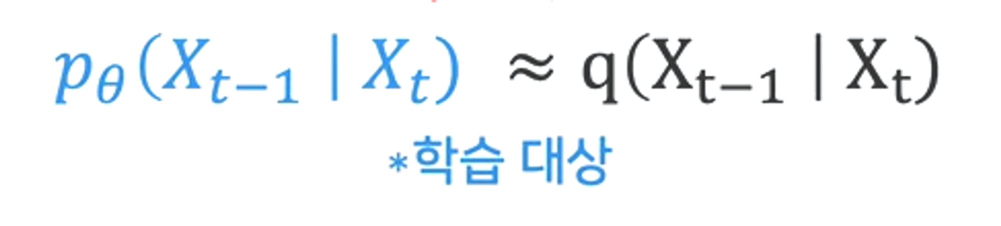
하지만, 노이즈가 추가된 데이터를 완벽하게 원래 상태로 되돌리는것은 불가능한 일이다. 

고로 Diffusion Model은 실제 분포 q($x_{t−1}$|$x_t$) 가 아닌 model의 가정을 만족하면서도 q($x_{t−1}$|$x_t$) 와 최대한 유사한 분포 $p_θ$($x_{t−1}$|$x_t$) 를 찾는다.

 

 

그럼 일단 기본적인 Diffusion Model 에 대한 소개는 여기까지 하도록 하고 이제 논문 내용을 정리해보겠다.

---

1. INTRODUCTION

• Image Synthesis 연구
  • Image Synthesis 는 최근 가장 많은 발전을 이룬 computer vision 분야 중 하나이며, 가장 큰 computational 수요를 가진 분야

• 기존 연구의 한계점
  • (GANs)
    • 복잡한 multi-modal distributions 으로 scale 하기 힘든 adversarial learning 으로 인해 제한된 variability 를 가진 data 에 국한됨. → 다양한 데이터에 적용하기 힘들다.
  • DMs
    • pixel space 에서 작동하기 때문에 powerful DMs 의 optimization 은 많은 GPU 가 필요하고 sequential evaluations 로 인해 긴 inference 시간이 필요

Democratizing High-Resolution Image Synthesis

• DM 의 compute resources
  • likelihood-based models 의 DM은 데이터의 디테일한 부분까지 모델링하는 mode-covering 동작으로 인해 과도한 compute resources 가 요구된다.
  • 모델을 training and evaluating 을 하기 위해서는 RGB 이미지의 고차원 공간에서 function evaluations (ex. gradient computations) 이 필요하고 이는 역시 많은 컴퓨팅 리소스가 필요하다.

 

결국 이 문제는 연구 커뮤니티와 사용자에게 두 가지 결과를 초래한다.

1. DM 을 학습시키기 위해서는 필드의 소수만이 사용할 수 있는 방대한 컴퓨팅 리소스가 필요하다. → 수많은 탄소발자국을 남긴다.
2. trained model 을 평가할 때에도 동일한 model architecture 를 순서대로 실행해야 하기 때문에 역시 많은 시간과 비용이 든다.

• 해결 방안
  • 컴퓨팅 리소스를 줄이고 모델의 접근성을 높이기 위해서는 training and sampling 모두 computational complexity 를 줄여야 함.

→ 결국 DM 의 성능을 유지하고 computational demands 를 줄이는 것이 고해상도 이미지 생성 연구 대중화의 핵심이다.

Departure to Latent Space

논문은 pixel space 에서 학습된 기존의 Diffusion Models 을 분석하는 것으로 시작된다.

 

Diffusion Models 의 대략적인 학습 단계는 다음과 같다.

• 학습 단계(two stages)
  1. perceptual compression stage 
     • high-frequency details 을 제거하지만 아직 semantic variation 은 학습하지 않음.
  2. semantic compression stage
     • 실제 generative model 이 데이터의 semantic and conceptual composition 학습함.

• perceptual and semantic compression 설명
  • digital image 의 대부분의 비트 : imperceptible details
  • DM은 responsible loss term 을 최소화하여 이러한 의미 없는 정보(imperceptible details) 를 제거하는 것이 가능하다. 그러나 (during training) gradients 및 neural network backbone (training and inference) 은 여전히 모든 pixel 에서 평가되어 과도한 computations 이 요구됨.

• perceptual and semantic compression 단계 정리
  • 한마디로 perceptual compression stage 의 경우 downsampling을 통해 의미 없는 정보를 제거한다는 뜻인 거 같다.두 번째인 semantic compression stage 에서는 downsampling을 통해 축소된 이미지 안에서 semantic 한 정보를 찾아 compression 한다는 의미인 듯

 

따라서 해당 논문의 목표는 perceptually equivalent + computationally suitable space 찾아서 high-resolution image synthesis 을 위한 diffusion models 을 훈련하는 것이다.

 

결국 Diffusion Model을 pixel space 가 아닌 pretrained autoencoders 의 latent space 에 적용하고 cross-attention layers 도입한 latent diffusion models (LDMs) 제안한다.

 

• About Latent Diffusion Models(LDMs)
  
  • autoencoder를 통해 perceptual compression을 수행한다.
  • lower dimensionality 인 compressed latent space 작동함으로써 2가지 단점을 해결한다. → 컴퓨팅 리소스 ⬇️ +synthesis quality 를 유지하면서도 inference speed ⬆️

autoencoder 는 data space 와 perceptually equivalent 하면서도 lower-dimensional representational space 제공하며 이를 통해 기존 연구들과 다르게 spatial compression 에 의존할 필요가 없다.

? : spatial dimensionality(공간적 차원; pixel space) 보다 더 좋은 scaling properties 을 가지고 있는 latent space 에서 DM 을 학습하기 때문에

3. Method

해당 논문은 autoencoding model 을 활용하여 generative learning phase / compression 을 분리하는 방법을 제안한다.

 

• autoencoding model
  • image space 와 인지적으로(perceptually) 동등한 space를 학습하면서도 computational complexity 를 크게 감소시킨다.
  • 장점 
    1. high-dimensional image space 에서 벗어나 low-dimensional space 에서 sampling 이 수행되므로 훨씬 효율적인 DMs를 얻을 수 있다.
    2. UNet architecture 기반의 DM 의 inductive bias 을 활용하여 spatial structure 를 가진 data 에 특히 효과적이다. → 기존 연구에서 요구하는 높은 spatial compression 을 완화한다.

3.1. Perceptual Image Compression (Pixel Space ↔ Latent Space)

논문의 perceptual compression 모델은 autoencoder(perceptual loss + a patch-based adversarial objective) 로 구성된다.

아래 사진의 pixel space(ε,D) 에 해당된다.

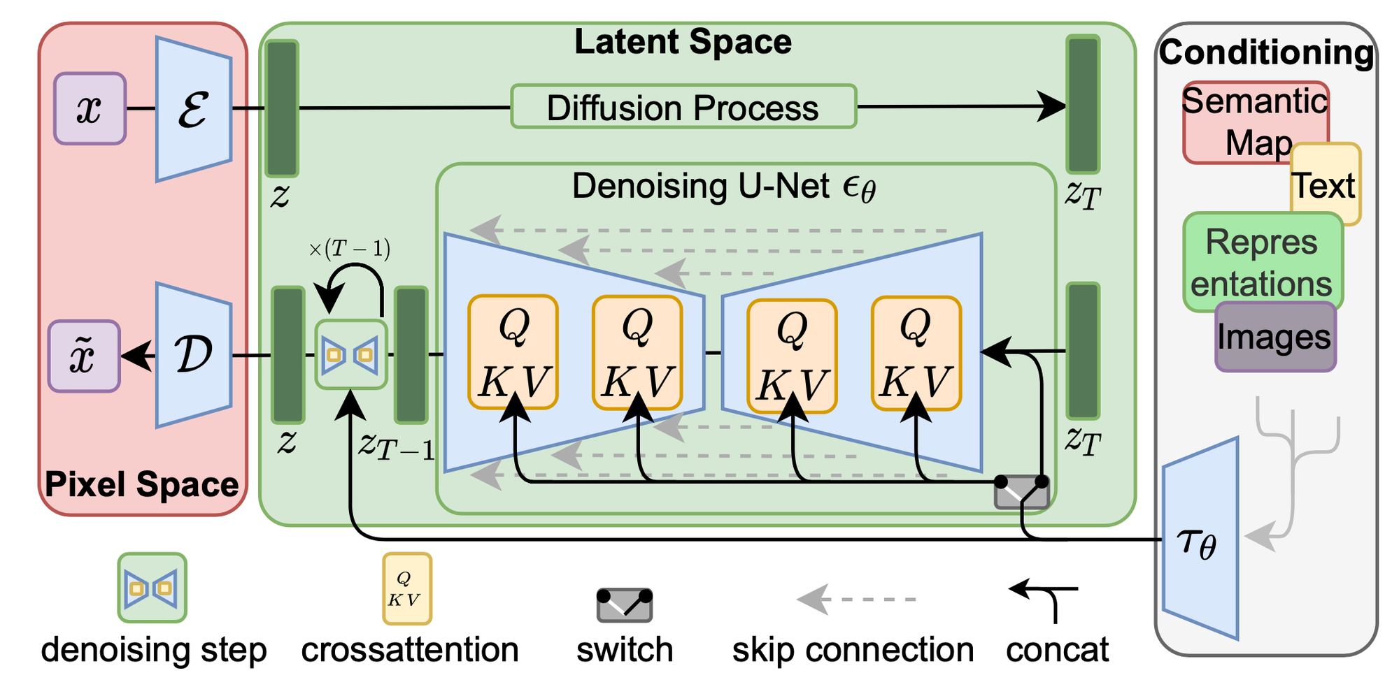
• 인코더(encoder) ε: x → z(latent representation)
• 디코더(decoder) D: z(latent representation) → x˜

data

• x ∈ R{H×W×3} : RGB 공간의 이미지
• encoder ε : x 를 latent representation z = ε(x)으로 인코딩 ⇒ x downsampling (factor f = H/h = W/w)
• z ∈ R{h×w×c} = ε(x) : latent representation (2-dimensional structure)
• decoder D : latent representation(z) 를 single pass로 decoding 하여 x˜ = D(z) = D(ε(x))를 제공
• x˜ = D(z) = D(E(x)) : reconstruction 이미지

결국 정리하면 encoder ε 는 고차원의 이미지(x)를 잘 표현하는 manifold 인 latent representation z 추출하고 decoder D는 latent representation z로 부터 reconstruction 이미지(x˜) 로 복원한다.

본 논문에서는 각기 다른 downsampling factor f = 2 m, m ∈ N 에 대해 실험했다고 한다.

3.2. Latent Diffusion Models

Diffusion Model objective

이 모델은 denoising autoencoder ϵ_θ(x_t,t); t=1,…,T 의 weighted sequence로 볼 수 있으며, noisy input x_t 로 부터 원본 이미지 x 를 predict하고자 한다.

 

• ϵ : noise, Forward diffusion process 를 진행할 때 사용한 실제 noise 값
• $ϵ_θ$ : denoising autoencoder
• $x_t$ : noised sample
• $t$ : noise level → $t-1, t-2,...,t$ 갈수록 less-noisy화 되는 것
• $ϵ_θ(x_t,t)$ : denoising process 의 noise

$L_{DM}$ 은 t 에서 t-1로 가기위해, [실제 noise - denoising process 의 noise] 라는 식의 결과 값을 줄여나가는 과정으로 loss minimize 하는 것이다.

즉, $L_{DM}$은 실제 분포와 근사한 분포를 만들어내기 위해 noising process 사용했던 noise ϵ 에 근사시키는 네트워크를 학습하는 것이다.

 

하지만 위의 식은 Latent space가 적용되지 않은 Diffusion Model의 objective이다.

Latent space가 적용된 LDM의 objective는 아래와 같다.

Generative Modeling of Latent Representations

LDMs은 ε와 D로 구성된 perceptual compression 모델을 통해 low-dimensional latent space에 접근할 수 있는데, 이는 likelihood-based 생성 모델에 더욱 적합하다고 한다.

 

• $ε$ : forward process가 고정되어 있기 때문에, $z_t$ 는 학습 과정에서 $ε$ 에 의해 쉽게 얻을 수 있다.
• $D$ : $p(z)$로 부터의 sample은 $D$를 통해 single pass로 쉽게 decoding 될 수 있다.

Latent Diffusion Model objective

• denoising model neural backbone $ϵ_θ(◦, t)$ : time-conditional UNet
• $x_t$ : noised sample → $z_t$ : noised latent representation(ε(x))

$L_{LDM}$ 도 마찬가지로 Diffusion Process($z$→$z_t$) 에서 사용했던 noise ϵ 에 근사시키는 네트워크를 학습하는 것이다.

3.3. Conditioning Mechanisms

semantic compression

LDM은 다양한 modalities 적용하기 위해 conditioning input y 도입했다.

diffusion model은 conditional distribution을 p(z|y)로 모델링 가능하다. 이것을 conditional denoising autoencoder $ϵ_θ$ ($z_t$ , $t$, $y$) 로 구현했는데, $ϵ_θ$는 이미지 생성을 위한 conditioning input y (text, semantic maps)를 컨트롤하거나, image-to-image translation task를 수행할 수 있다.

 

BUT, conditioning input $y$를 denoising autoencoder $ϵ_θ$에 적용하기 위해서는 preprocessing 필요하다.

 

preprocessing을 하기 위해 domain specific encoder $τ_θ$를 도입한다.

이러한 $τ_θ$는 conditioning input $y$를 다양한 modalities(language prompts, semantic 맵과 같은)로부터 전처리할 수 있다고 한다.

 

• domain specific encoder $τ_θ$ : conditioning input y → intermediate representation $τ_θ(y)$ ∈ $R^{M×d_τ}$ 로 project 한다.

결국 $ϵ_θ$의 intermediate layers에 적합하게 encoding됨으로써 semantic compression을 수행하게 된다. 

conditional denoising autoencoder $ϵ_θ$ ($z_t$ , $t$, $y$)

denoising model $ϵ_θ(◦, t)$ 의 neural backbone 은 오른쪽 사진과 같은 time-conditional UNet structure 이다.

이 네트워크 구조를 활용하여 이미지의 위치와 특징을 추출하기 위해 인코더 레이어와 디코더 레이어의 직접 연결하는 skip connection 과 concatenation을 통해 인코딩 단계의 각 레이어에서 얻은 특징을 디코딩 단계의 각 레이어에 합친다.

 

$ϵ_θ$ intermediate layers은 UNet backbone을 다양한 input modality에 대해 conditioning 할 수 있도록 cross-attention mechanism 적용했다.

즉, cross-attention mechanism 을 통해 다양한 input modality 를 model 에 적용할 수 있다.

 

• UNet 의 intermediate layers : cross-attention layer 로 구성

여기서 Attention 이란 Attention(Q, K, V) = softmax$(\frac{QK^T}{\sqrt{d}}) · V$이 구현되어 있으며, softmax를 통해 얻은 어텐션 분포 값에 value 값을 곱해서 어텐션 값을 얻는다. 즉, 예측해야 할 값과 연관이 있는 input 부분에 더 집중해서 참고하는 전형적인 어텐션 연산이 이루어진다.

 

또한 cross attention은 2 개의 embedding sequences 간의 correlation 학습하는 것이다.

input은 Query, Key, Value를 받고 위 사진처럼 key, value 의 경우 같은 sequence 에서 얻지만, query는 다른 sequence에서 얻는다.(즉, query 출처 ≠ key, value 출처)

 

$ϵ_θ$ 의 Q, K, V

이 개념을 LDM에 적용해보자면 여기서 예측해야 할 값인 쿼리(Q)는 $φ_i$($z_t$) 즉, encoder $ϵ_θ$ 을 구현하는 UNet 의 intermediate representation 이고, 키(K)와 벨류(V)는 모두 $τ_θ$ 에 y를 넣어 인코딩한 $τ_θ$(y) 이다.

 

결과적으로 LDM 의 cross attention은 unet 의 중간층 representation를 생성할 때, conditioning input y 의 어떤 정보를 Attention 해야할지 파악하는 과정이다.

즉, 이 과정을 통해 conditioning input y를 참고해서 noised latent representation $z_t$ 를 denoising 할 수 있게 된다.

conditional Latent Diffusion Model objective

conditioning 까지 적용한 Latent Diffusion Model objective는 아래 식과 같다.

• $τ_θ$ , $ϵ_θ$ : Eq. 3 을 통해 optimized

denoising 과정을 수행할때 image-conditioning pairs [$z_t$-$τ_θ(y)$] 를 기반으로 노이즈를 줄여나가는 작업을 진행한다.

autoencoder loss (perceptual loss + a patch-based adversarial objective)

또한, 해당 논문에서는 perceptual compression을 수행하는 autoencoder의 objective도 정의하고 있는데 따로 식이 있거나 하진 않다.

 

• perceptual loss: feature map 거리 계산
• patch based adversarial objective: patch 단위로 T/F를 판별하는 방식

득히 patch based adversarial objective를 통해 local realism 실현할 수 있고 reconstruction 결과물이 image manifold 에만 국한되도록 보장할 수 있다고 한다.

 

LDM process

1. perceptual compression ε: x → latent representation z = ε(x) (latent space에 매핑)
2. diffusion process: latent representation z → $z_T$(noised latent representation)
3. conditioning mechanism & semantic compression $τ_θ$: conditioning input y → intermediate representation $τ_θ$(y)
4. denoising process: $τ_θ$(y)를 참고하여 noised latent representation $z_T$ → latent representation z
5. perceptual compression D: latent representation z →  reconstruction 이미지 x˜ = D(z)

사실 LDM task 는 꼭 복원(reconstruction)만 수행할 수 있는 것은 아니다. text-image synthesis 와 layout-to-image synthesis 와 같은 다양한 작업을 할 수 있는데 이때는 switch를 통해 perceptual compression ε(1번 과정) 과 diffusion process(2번 과정)는 생략할 수 있다.

 

4. Experiments

• train dataset

4.1. On Perceptual Compression Tradeoffs

• class-conditional LDMs 의 sample quality

ImageNet dataset 으로 training progress(2M train steps) 를 걸쳐 각기 다른 downsampling factors f 를 적용한 모델을 비교한다.

4.2. Image Generation with Latent Diffusion

• < layout-to-image, Text-To-Image>

• text-to-image modeling,

1. BERT-tokenizer 를 사용하고 τθ을 transformer 로 구현하여 cross-attention 을 통해 UNet latent code 를 생성한다.
2. [language representation ↔ visual synthesis] 를 학습하기 위한 domain specific encoder $τ_θ$는 user-defined text prompts 로 일반화

4.3. Conditional Latent Diffusion

• Convolutional Sampling Beyond $256^2$

4.4. Super-Resolution with Latent Diffusion

• ImageNet 64→256 super-resolution on ImageNet-Val.

4.5. Inpainting with Latent Diffusion

 

 

 

 

[original paper] : https://arxiv.org/abs/2112.10752

High-Resolution Image Synthesis with Latent Diffusion Models

 

[reference]

- LDM 리뷰-

https://lilianweng.github.io/posts/2021-07-11-diffusion-models/

https://jang-inspiration.com/latent-diffusion-model

https://towardsdatascience.com/what-are-stable-diffusion-models-and-why-are-they-a-step-forward-for-image-generation-aa1182801d46

 

- DM 설명-

https://americanoisice.tistory.com/109

https://blog.mnc.ai/48